Not all passengers who buy a plane ticket show up at boarding. The no shows make flights occur with idle capacity and incur an opportunity cost for the operator. To compensate, airlines use overbooking (sale of seats above the flight capacity). But how many additional seats should we offer without it becoming a chronic passenger relocation problem?
By overbooking, the risk has more passengers than the plane can handle at the time of boarding, leading to higher costs to relocate passengers on other flights and causing wear on the brand through user dissatisfaction. In this post, we will analyze the demand distribution and the behavior of the no shows to find the best overbooking strategy through Monte Carlo simulation to establish a statistically secure overbooking policy.
Approach
The approach we will use to try to find the best overbooking strategy will follow these steps:
Understand and model the behavior (distribution) of demand
Simulate boarding situations using Monte Carlo
Define an overbooking strategy based on the probability of passenger relocation
Flight Demand Data
As a starting point, we will load the demand and attendance data of a particular commercial flight available in this excel sheet and briefly explore the data and try to understand the behavior of the demand so that it can be modeled.
 1
 2
 3
 4
 5
 6
 7
 8
 9
10
11
12
13
14
15
16
# setup ####library(tidyverse)# read data ####raw_data<-readxl::read_xlsx("./assets/Flight-Overbooking-Data.xlsx")# simple clean upflight_dt<-raw_data%>%dplyr::select(1:5)%>%janitor::clean_names()# glimpseflight_dt%>%head(10)%>%knitr::kable()%>%kableExtra::kable_styling(font_size=11)
date
demand
booked
shows
rate
2014-01-01
132
132
117
0.8863636
2014-01-02
154
150
142
0.9466667
2014-01-03
142
142
126
0.8873239
2014-01-04
152
150
141
0.9400000
2014-01-05
162
150
142
0.9466667
2014-01-06
146
146
131
0.8972603
2014-01-07
134
134
118
0.8805970
2014-01-08
158
150
140
0.9333333
2014-01-09
165
150
138
0.9200000
2014-01-10
156
150
139
0.9266667
It is a very simple and straightforward dataset containing information on the date, the demand, how many passengers were registered, how many showed up, and the attendance rate (appeared/registered).
Data Overview
1
2
3
# overviewflight_dt%>%skimr::skim()
Table 1: Data summary
Name
Piped data
Number of rows
730
Number of columns
5
_______________________
Column type frequency:
numeric
4
POSIXct
1
________________________
Group variables
None
Variable type: numeric
skim_variable
n_missing
complete_rate
mean
sd
p0
p25
p50
p75
p100
hist
demand
0
1
150.40
12.28
117.00
142.0
150.00
158.00
191.00
▁▆▇▂▁
booked
0
1
145.32
6.85
117.00
142.0
150.00
150.00
150.00
▁▁▁▂▇
shows
0
1
133.73
9.10
106.00
127.0
138.00
141.00
147.00
▁▂▃▂▇
rate
0
1
0.92
0.03
0.88
0.9
0.92
0.94
0.99
▇▃▇▃▁
Variable type: POSIXct
skim_variable
n_missing
complete_rate
min
max
median
n_unique
date
0
1
2014-01-01
2015-12-31
2014-12-31 12:00:00
730
As you can see, there is an upper limit of 150 in the registered column, indicating that this is the capacity of the flight, that is, 150 seats.
Demand Behavior
Let’s try to model the demand, making the fit of your distribution, for we will use the package {fitdistrplus}.
1
2
3
4
library(fitdistrplus)# checking the empirical distributionplotdist(flight_dt$demand,discrete=T)
1
2
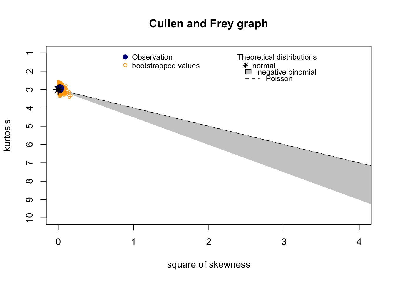
# what are the distribution candidates?descdist(flight_dt$demand,boot=1000,discrete=T)
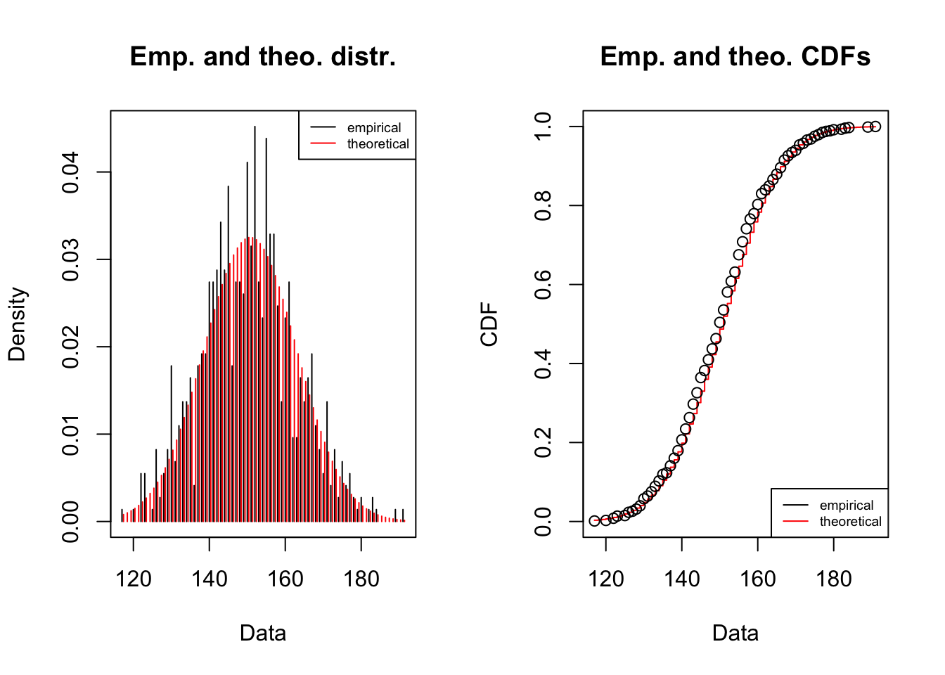
The {fitdistrplus} package indicated three candidates as the best fit for the demand distribution: normal, poisson or negative binomial. Let’s test which of the two most common ones has the best fit.
Normal Distribution
1
2
3
4
# lets fit a normal and see what we getfitdist(flight_dt$demand,"norm",discrete=T)%T>%plot()%>%summary()
1
2
3
4
5
6
7
8
9
10
## Fitting of the distribution ' norm ' by maximum likelihood
## Parameters :
## estimate Std. Error
## mean 150.39726 0.4540115
## sd 12.26672 0.3210346
## Loglikelihood: -2865.855 AIC: 5735.709 BIC: 5744.895
## Correlation matrix:
## mean sd
## mean 1 0
## sd 0 1
Poisson Distribution
1
2
3
4
# lets fit a poisson and see what we getfitdist(flight_dt$demand,"pois",discrete=T)%T>%plot()%>%summary()
1
2
3
4
5
## Fitting of the distribution ' pois ' by maximum likelihood
## Parameters :
## estimate Std. Error
## lambda 150.3973 0.4538983
## Loglikelihood: -2864.742 AIC: 5731.484 BIC: 5736.077
Melhor modelo
We observed that the Poisson distribution has, marginally, the best fit monitoring the indicators [loglikehood](https://www.statology.org › likelihood-vs-probability), IAC and [BIC](https:/ /en.wikipedia.org/wiki/Bayesian_information_criterion). So let’s use poisson as our distribution model for demand.
1
2
# Emp CDF fit for Poisson is a little better and IAC also is marginally betterdemand.pois<-fitdist(flight_dt$demand,"pois",discrete=T)
Attendance
The show up can be modeled as a binomial lottery over the number of registered passengers for the flight with a success rate determined by the historical average.
1
mean(flight_dt$rate)
1
## [1] 0.9194333
We found that the historical average presence rate for the flight is 92%, we can use this information to simulate the presence process by doing:
1
2
3
pass_reg<-145# number of passengers registered for the fligthshow_ups<-rbinom(1,pass_reg,mean(flight_dt$rate))# one random binomial draw with size of pass_reg at historic show_up rateshow_ups
1
## [1] 127
Simulation Model
We are going to make a model to simulate a boarding situation, in this first model, we will establish a fixed number for the overbooking of 15 positions, i. e., we will offer 15 additional seats for sale in addition to the flight capacity (150 positions).
# demand simulationsimulateDemand<-function(overbook,n,capacity,showup_rate,demand_model){# generate the demand scenarios (pois distributed)tibble(demand=rpois(n,demand_model$estimate))%>%# booked: demand inside capacity+overbook (flight seats) mutate(booked=map_dbl(demand,~min(.x,overbook+capacity)))%>%# show-ups and no showsmutate(shows=map_dbl(booked,~rbinom(1,.x,showup_rate)),no_shows=booked-shows)%>%# shop-up ratemutate(showup_rate=shows/booked)%>%# calc overbook and empty seatsmutate(overbooked=shows-capacity,empty_seats=capacity-shows)%>%# remove negative valuesmutate(overbooked=map_dbl(overbooked,~max(.x,0)),empty_seats=map_dbl(empty_seats,~max(.x,0)))%>%return()}# simulating 10 thousand cases using:# fligth capacity: 150 passengers# overbooking: 15 positions# show_up rate: ~92% historic based# poisson distribuion: fitted previouslysim<-simulateDemand(15,10000,150,mean(flight_dt$rate),demand.pois)# what we gotsim%>%head(10)%>%knitr::kable()%>%kableExtra::kable_styling(font_size=11)
demand
booked
shows
no_shows
showup_rate
overbooked
empty_seats
138
138
129
9
0.9347826
0
21
156
156
140
16
0.8974359
0
10
130
130
121
9
0.9307692
0
29
157
157
142
15
0.9044586
0
8
148
148
132
16
0.8918919
0
18
131
131
117
14
0.8931298
0
33
154
154
142
12
0.9220779
0
8
163
163
147
16
0.9018405
0
3
165
165
142
23
0.8606061
0
8
137
137
125
12
0.9124088
0
25
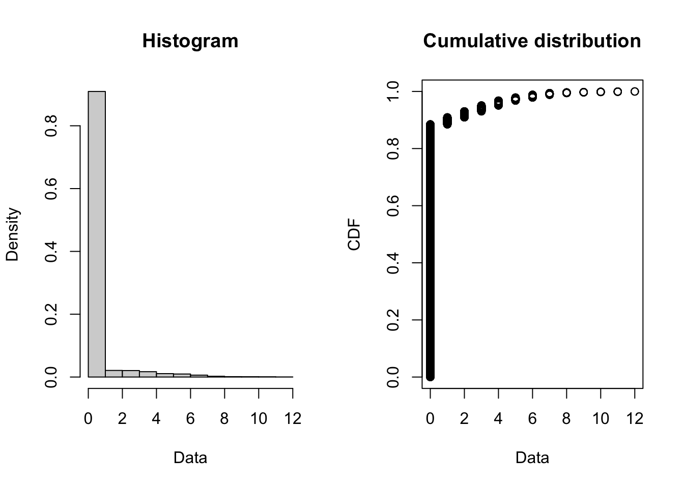
With a model to simulate a boarding situation, we can analyze the behavior of the frequency of the real overbooking (that is) how many passengers, above the actual capacity of the plane (150 seats), appear at the boarding gate and who would need to be relocated to other flights (or financially compensated).
1
2
3
4
5
# lets visualize the overbooked passengers distributionsim%>%count(overbooked)%>%knitr::kable()%>%kableExtra::kable_styling(font_size=11)
overbooked
n
0
8848
1
245
2
210
3
206
4
170
5
108
6
96
7
60
8
24
9
12
10
10
11
8
12
3
1
plotdist(sim$overbooked)
Overbooking Policy
With the view of how real overbooking behaves (# of reassigned passengers), we can then establish an overbooking policy, for example, establishing that in 95% of the boarding situations of this flight, the number of relocated passengers does not exceed 2. So in this scenario of 15 additional accents, we would have
1
2
3
4
5
6
7
8
# chance to have 2 or less bumped passbumped_more_2<-sim%>%count(overbooked)%>%filter(overbooked>2)%>%summarise(total=sum(n))%>%unlist()1-(bumped_more_2/10000)
1
2
## total
## 0.9303
It would not be possible to meet this criterion with 15 additional seats in this demand profile and attendance behavior, so how many seats should we offer to meet the established policy?
Simulating Overbooking
Let’s then analyze what would be the number of additional positions to be offered that allow the company to stay within the overbooking policy defined above. To do that, we simulate various boarding situations providing different additional seats (above the flight capacity), going, for example, from 1 to 20 extra positions.
# lets find the optimal overbook to get max of 2 bumped passengers in 95% of situations# before that, lets create a auxiliary functionprobBumpedPass<-function(simulation,nPass){# calc the probability of the number of bumped passengers be less then nPass in a simulationsimulation%>%count(overbooked)%>%filter(overbooked<=nPass)%>%summarise(total=sum(n)/10000)%>%unlist()%>%return()}# looking the behavior of the probability to get 2 (or 5) less passengers bumpedtibble(overbook=1:20)%>%mutate(simulation=map(overbook,simulateDemand,n=10000,capacity=150,showup_rate=mean(flight_dt$rate),demand_model=demand.pois))%>%mutate(prob2BumpPass=map_dbl(simulation,probBumpedPass,nPass=2),prob5BumpPass=map_dbl(simulation,probBumpedPass,nPass=5))%>%pivot_longer(cols=c(-overbook,-simulation),names_to="bumped",values_to="prob")%>%ggplot(aes(x=overbook,y=prob,color=bumped))+geom_hline(yintercept=0.95,linetype="dashed")+geom_vline(xintercept=13,linetype="dashed",color="pink")+geom_vline(xintercept=18,linetype="dashed",color="lightblue")+geom_line()+geom_point()+labs(title="Bumped Passengers",subtitle="Chance to bump until 2 passengers (red) or 5 passengers (blue)",y="probability",x="seats offered beyond flight capacity")+theme_light()
We can see that by offering 13 additional seats, we would be able to meet the policy of having more than two reassigned passengers on only 5% of flights. If the policy were a 95% chance of having five or less, we could offer 18 seats in overbooking.
Dependency between demand and show-up rate
We had assumed a constant show-up rate, no matter the demand for a flight on a given day, i.e., boarding attendance follows a constant rate. But is this hypothesis true?
1
2
# we assume that the showup rate is fixed, is it?cor.test(flight_dt$demand,flight_dt$rate)
 1
 2
 3
 4
 5
 6
 7
 8
 9
10
11
##
## Pearson's product-moment correlation
##
## data: flight_dt$demand and flight_dt$rate
## t = 26.194, df = 728, p-value < 2.2e-16
## alternative hypothesis: true correlation is not equal to 0
## 95 percent confidence interval:
## 0.6572186 0.7321212
## sample estimates:
## cor
## 0.6965629
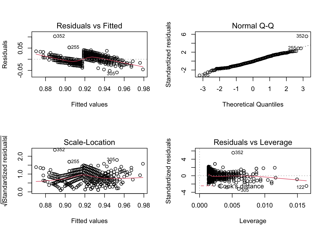
This correlation rate is too high to ignore. Let’s redo the boarding model considering this dependence, incorporating a linear dependence model between attendance rate and demand.
1
2
3
4
5
# lets make a simple linear modelrate_model<-lm(rate~demand,data=flight_dt)# what we got?summary(rate_model)
1
2
3
4
5
6
7
8
9
10
11
12
13
14
15
16
17
18
##
## Call:
## lm(formula = rate ~ demand, data = flight_dt)
##
## Residuals:
## Min 1Q Median 3Q Max
## -0.059294 -0.013465 -0.001671 0.013015 0.102829
##
## Coefficients:
## Estimate Std. Error t value Pr(>|t|)
## (Intercept) 6.986e-01 8.460e-03 82.57 <2e-16 ***
## demand 1.469e-03 5.606e-05 26.19 <2e-16 ***
## ---
## Signif. codes: 0 '***' 0.001 '**' 0.01 '*' 0.05 '.' 0.1 ' ' 1
##
## Residual standard error: 0.01858 on 728 degrees of freedom
## Multiple R-squared: 0.4852, Adjusted R-squared: 0.4845
## F-statistic: 686.1 on 1 and 728 DF, p-value: < 2.2e-16
1
2
par(mfrow=c(2,2))plot(rate_model)
1
par(mfrow=c(1,1))
Let’s change the function that does the simulation by incorporating the dependency model.
# another simulation model considering the dependency between showup rate and demandsimulateDemandShowUpModel<-function(overbook,n,capacity,showup_model){# generate a demand simulationdemSim<-tibble(demand=rpois(n,demand.pois$estimate))# based in showup model calc a predicted showup_rate for each demanddemSim$predShowup_rate=predict(showup_model,newdata=demSim)# complete the simulationdemSim%>%# booked: demand inside capacity (flight seats) mutate(booked=map_dbl(demand,~min(.x,overbook+capacity)))%>%# compute the show-ups and no showsmutate(shows=map2_dbl(booked,predShowup_rate,~rbinom(1,.x,.y)),no_shows=booked-shows)%>%# shop-up ratemutate(showup_rate=shows/booked)%>%# calc overbook and empty seatsmutate(overbooked=shows-capacity,empty_seats=capacity-shows)%>%# remove negative valuesmutate(overbooked=map_dbl(overbooked,~max(.x,0)),empty_seats=map_dbl(empty_seats,~max(.x,0)))%>%return()}# simulating one case ####sim<-simulateDemandShowUpModel(15,10000,150,rate_model)# what we gotsim%>%head(10)%>%knitr::kable()%>%kableExtra::kable_styling(font_size=11)
demand
predShowup_rate
booked
shows
no_shows
showup_rate
overbooked
empty_seats
166
0.9423470
165
156
9
0.9454545
6
0
167
0.9438155
165
151
14
0.9151515
1
0
175
0.9555641
165
162
3
0.9818182
12
0
145
0.9115070
145
135
10
0.9310345
0
15
156
0.9276613
156
147
9
0.9423077
0
3
154
0.9247241
154
144
10
0.9350649
0
6
166
0.9423470
165
154
11
0.9333333
4
0
171
0.9496898
165
159
6
0.9636364
9
0
173
0.9526269
165
157
8
0.9515152
7
0
131
0.8909471
131
123
8
0.9389313
0
27
1
2
3
4
5
6
# lets visualize the overbooked passengers distributionsim%>%count(overbooked)%>%head(10)%>%knitr::kable()%>%kableExtra::kable_styling(font_size=11)
overbooked
n
0
8040
1
208
2
197
3
196
4
214
5
209
6
199
7
189
8
172
9
121
1
plotdist(sim$overbooked)
We can see that the distribution (for this case of 15 additional accents) spreads out a bit. Now, there are more chances of rearrangement by overbooking, apparently.
1
2
3
4
5
6
7
8
# chance to have 2 or less bumped passbumped_more_2_dep<-sim%>%count(overbooked)%>%filter(overbooked>2)%>%summarise(total=sum(n))%>%unlist()bumped_more_2_dep
1
2
## total
## 1555
And arguably, only 84% of having two or fewer passengers relocated in this scenario, compared to 93% of the previous scenario. Let’s redo the simulation considering various strategies for overbooking, as we did in the previous model.
1
2
3
4
5
6
7
8
9
10
11
12
13
14
15
16
17
# looking the behavior of the probability to get 2 (or 5) less passengers bumped# in the new modeltibble(overbook=1:20)%>%mutate(simulation=map(overbook,simulateDemandShowUpModel,n=10000,capacity=150,showup_model=rate_model))%>%mutate(prob2BumpPass=map_dbl(simulation,probBumpedPass,nPass=2),prob5BumpPass=map_dbl(simulation,probBumpedPass,nPass=5))%>%pivot_longer(cols=c(-overbook,-simulation),names_to="bumped",values_to="prob")%>%ggplot(aes(x=overbook,y=prob,color=bumped))+geom_hline(yintercept=0.95,linetype="dashed")+geom_vline(xintercept=8,linetype="dashed",color="pink")+geom_vline(xintercept=12,linetype="dashed",color="lightblue")+geom_line()+geom_point()+labs(title="Bumped Passengers (show-up rate dependent)",subtitle="Chance to bump until 2 passengers (red) or 5 passengers (blue)",y="probability",x="seats offered beyond flight capacity")+theme_light()
We get significantly different results when considering that the show-up rate is demand-dependent, so we need to offer far fewer additional seats to maintain an eventual policy of 95% of flights with two or fewer reassigned passengers.
Results for deploying the overbooking policy:
To have two or fewer passengers relocated on 95% of flights: 8 additional seats
To have five or fewer passengers relocated on 95% of flights: 12 additional seats