Some generic data visualization using ggplot2 package and UK Bakeoff data.
This is a simple post of some visualization exercises using {ggplot2} and the data from Great British Bakeoff TV show from Alison Hill, Chester Ismay, and Richard Iannone.
Load Data
1
2
|
library(bakeoff)
library(tidyverse)
|
Data Overview
1
2
|
bakeoff::bakers %>%
  head(10)
|
 1
 2
 3
 4
 5
 6
 7
 8
 9
10
11
12
13
14
15
16
17
18
19
20
|
## # A tibble: 10 × 24
## series baker star_…¹ techn…² techn…³ techn…⁴ techn…⁵ techn…⁶ techn…⁷ serie…⁸
## <dbl> <chr> <int> <int> <int> <int> <dbl> <dbl> <dbl> <int>
## 1 1 Annet… 0 0 1 1 2 7 4.5 0
## 2 1 David 0 0 1 3 3 8 4.5 0
## 3 1 Edd 0 2 4 1 1 6 2 1
## 4 1 Jasmi… 0 0 2 2 2 5 3 0
## 5 1 Jonat… 0 1 1 2 1 9 6 0
## 6 1 Lea 0 0 0 1 10 10 10 0
## 7 1 Louise 0 0 0 1 4 4 4 0
## 8 1 Mark 0 0 0 0 NA NA NA 0
## 9 1 Miran… 0 2 4 1 1 8 3 0
## 10 1 Ruth 0 0 2 2 2 5 3.5 0
## # … with 14 more variables: series_runner_up <int>,
## # total_episodes_appeared <dbl>, first_date_appeared <date>,
## # last_date_appeared <date>, first_date_us <date>, last_date_us <date>,
## # percent_episodes_appeared <dbl>, percent_technical_top3 <dbl>,
## # baker_full <chr>, age <dbl>, occupation <chr>, hometown <chr>,
## # baker_last <chr>, baker_first <chr>, and abbreviated variable names
## # ¹star_baker, ²technical_winner, ³technical_top3, ⁴technical_bottom, …
|
1
2
|
bakeoff::challenges %>%
  head(10)
|
 1
 2
 3
 4
 5
 6
 7
 8
 9
10
11
12
13
14
|
## # A tibble: 10 × 7
## series episode baker result signature techn…¹ shows…²
## <int> <int> <chr> <chr> <chr> <int> <chr>
## 1 1 1 Annetha IN "Light Jamaican Black Cakewi… 2 Red, W…
## 2 1 1 David IN "Chocolate Orange Cake" 3 Black …
## 3 1 1 Edd IN "Caramel Cinnamon and Banana… 1 <NA>
## 4 1 1 Jasminder IN "Fresh Mango and Passion Fru… NA <NA>
## 5 1 1 Jonathan IN "Carrot Cake with Lime and C… 9 Three …
## 6 1 1 Louise IN "Carrot and Orange Cake" NA Never …
## 7 1 1 Miranda IN "Triple Layered Brownie Meri… 8 Three …
## 8 1 1 Ruth IN "Three Tiered Lemon Drizzle … NA Classi…
## 9 1 1 Lea OUT "Cranberry and Pistachio Cak… 10 Raspbe…
## 10 1 1 Mark OUT "Sticky Marmalade Tea Loaf" NA Heart-…
## # … with abbreviated variable names ¹technical, ²showstopper
|
1
2
|
bakeoff::episodes %>%
  head(10)
|
 1
 2
 3
 4
 5
 6
 7
 8
 9
10
11
12
13
14
15
16
|
## # A tibble: 10 × 10
## series episode bakers_appea…¹ baker…² baker…³ star_…⁴ techn…⁵ sb_name winne…⁶
## <dbl> <dbl> <int> <int> <int> <int> <int> <chr> <chr>
## 1 1 1 10 2 8 0 1 <NA> <NA>
## 2 1 2 8 2 6 0 1 <NA> <NA>
## 3 1 3 6 1 5 0 1 <NA> <NA>
## 4 1 4 5 1 4 0 1 <NA> <NA>
## 5 1 5 4 1 3 0 1 <NA> <NA>
## 6 1 6 3 0 3 0 0 <NA> Edd
## 7 2 1 12 1 11 1 1 Holly <NA>
## 8 2 2 11 1 10 1 1 Jason <NA>
## 9 2 3 10 2 8 1 1 Yasmin <NA>
## 10 2 4 8 1 7 2 1 Holly,… <NA>
## # … with 1 more variable: eliminated <chr>, and abbreviated variable names
## # ¹bakers_appeared, ²bakers_out, ³bakers_remaining, ⁴star_bakers,
## # ⁵technical_winners, ⁶winner_name
|
1
2
|
bakeoff::ratings %>%
  head(10)
|
 1
 2
 3
 4
 5
 6
 7
 8
 9
10
11
12
13
14
15
16
|
## # A tibble: 10 × 11
## series episode uk_airdate viewers_7…¹ viewe…² netwo…³ chann…⁴ bbc_i…⁵ episo…⁶
## <dbl> <dbl> <date> <dbl> <dbl> <dbl> <dbl> <dbl> <dbl>
## 1 1 1 2010-08-17 2.24 7 NA NA NA 1
## 2 1 2 2010-08-24 3 3 NA NA NA 2
## 3 1 3 2010-08-31 3 2 NA NA NA 3
## 4 1 4 2010-09-07 2.6 4 NA NA NA 4
## 5 1 5 2010-09-14 3.03 1 NA NA NA 5
## 6 1 6 2010-09-21 2.75 1 NA NA NA 6
## 7 2 1 2011-08-16 3.1 2 NA NA NA 7
## 8 2 2 2011-08-23 3.53 2 NA NA NA 8
## 9 2 3 2011-08-30 3.82 1 NA NA NA 9
## 10 2 4 2011-09-06 3.6 1 NA NA NA 10
## # … with 2 more variables: us_season <dbl>, us_airdate <chr>, and abbreviated
## # variable names ¹viewers_7day, ²viewers_28day, ³network_rank,
## # ⁴channels_rank, ⁵bbc_iplayer_requests, ⁶episode_count
|
Data Characterization
1
|
skimr::skim(bakeoff::ratings)
|
Table: Table 1: Data summary
|
|
| Name |
bakeoff::ratings |
| Number of rows |
94 |
| Number of columns |
11 |
| _______________________ |
|
| Column type frequency: |
|
| character |
1 |
| Date |
1 |
| numeric |
9 |
| ________________________ |
|
| Group variables |
None |
Variable type: character
| skim_variable |
n_missing |
complete_rate |
min |
max |
empty |
n_unique |
whitespace |
| us_airdate |
49 |
0.48 |
12 |
18 |
0 |
39 |
0 |
Variable type: Date
| skim_variable |
n_missing |
complete_rate |
min |
max |
median |
n_unique |
| uk_airdate |
0 |
1 |
2010-08-17 |
2019-10-29 |
2015-08-22 |
94 |
Variable type: numeric
| skim_variable |
n_missing |
complete_rate |
mean |
sd |
p0 |
p25 |
p50 |
p75 |
p100 |
hist |
| series |
0 |
1.00 |
5.77 |
2.77 |
1.00e+00 |
3.25 |
6.00 |
8.00 |
1.000e+01 |
▆▇▇▇▇ |
| episode |
0 |
1.00 |
5.29 |
2.83 |
1.00e+00 |
3.00 |
5.00 |
8.00 |
1.000e+01 |
▇▇▇▇▆ |
| viewers_7day |
0 |
1.00 |
8.58 |
3.27 |
2.24e+00 |
6.61 |
8.97 |
10.27 |
1.590e+01 |
▃▂▇▂▂ |
| viewers_28day |
1 |
0.99 |
6.41 |
5.09 |
1.00e+00 |
1.00 |
8.98 |
9.93 |
1.603e+01 |
▇▁▅▂▂ |
| network_rank |
24 |
0.74 |
2.87 |
4.61 |
1.00e+00 |
1.00 |
1.00 |
1.00 |
1.800e+01 |
▇▁▁▁▁ |
| channels_rank |
44 |
0.53 |
2.02 |
1.12 |
1.00e+00 |
1.00 |
2.00 |
3.00 |
4.000e+00 |
▇▂▁▅▂ |
| bbc_iplayer_requests |
74 |
0.21 |
1862700.00 |
260983.38 |
1.37e+06 |
1715750.00 |
1915500.00 |
1985250.00 |
2.314e+06 |
▃▂▇▇▃ |
| episode_count |
0 |
1.00 |
47.50 |
27.28 |
1.00e+00 |
24.25 |
47.50 |
70.75 |
9.400e+01 |
▇▇▇▇▇ |
| us_season |
44 |
0.53 |
3.00 |
1.43 |
1.00e+00 |
2.00 |
3.00 |
4.00 |
5.000e+00 |
▇▇▇▇▇ |
Exploring some visualizations
Audience along episodes and seasons
 1
 2
 3
 4
 5
 6
 7
 8
 9
10
11
12
13
14
15
16
17
18
|
ep_df <- bakeoff::ratings %>%
  arrange(series, episode) %>%
  mutate(ep_id = row_number(),
         series = factor(series, ordered = T)) %>%
  select(ep_id, viewers_7day, series, episode)

series_label <- ep_df %>%
  group_by(series) %>%
  summarise(label_pos_x = mean(ep_id),
         label_pos_y = median(viewers_7day) + 1)

ep_df %>%
  ggplot(aes(x=ep_id, y=viewers_7day, fill=series)) +
  geom_col(color="white",alpha=.8, show.legend = F, size=.1) +
  geom_text(data=series_label, mapping=aes(x=label_pos_x, y=label_pos_y, label=series)) +
  theme_minimal() +
  labs(x="episodes", y="weekly viewers (millions)",
       title = "TV Show Audience")
|

 1
 2
 3
 4
 5
 6
 7
 8
 9
10
11
12
13
14
15
16
17
18
19
|
ep_df %>%
  group_by(series) %>%
  mutate( season_avg = mean(viewers_7day) ) %>%
  ungroup() %>%
  filter( series > 2) %>%
  ggplot(aes(x=episode, viewers_7day, color=viewers_7day)) +
  geom_point(alpha=.8)+
  geom_hline(aes(yintercept=season_avg)) +
  geom_segment(aes(xend=episode, yend=season_avg)) +
  # scale_color_gradient(low = "darkblue", high = "orange") +
  scale_color_viridis_c(option="plasma", begin = 0, end = .8, guide = FALSE) +
  scale_x_continuous(breaks = 1:10) +
  facet_wrap(~series, nrow = 2) +
  lims(y=c(0,NA)) +
  theme_light() +
  theme(legend.position = "none",panel.grid.minor = element_blank())  +
  labs(x="episodes", y="weekly viewers (millions)",
       title = "TV Show Audience Along the Seasons",
       subtitle = "Episodes vs Season Meen")
|

 1
 2
 3
 4
 5
 6
 7
 8
 9
10
11
12
13
14
15
16
17
18
19
20
|
series_label <- ep_df %>%
  group_by(series) %>%
  filter(episode==max(episode)) %>%
  mutate(
    position_x = episode+.1,
    position_y = viewers_7day
  )

ep_df %>%
  ggplot(aes(x=episode, y=viewers_7day, color=series, group=series)) +
  geom_line(alpha=.8, show.legend = F) +
  geom_text(data=series_label, aes(
    label=series,
    x=position_x,
    y=position_y
  ), show.legend = F) +
  scale_color_discrete() +
  theme_light()  +
  labs(x="episodes", y="weekly viewers (millions)",
       title = "Audience Progression along each season")
|

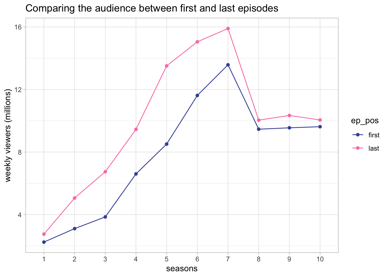
Comparing audience between first and last episodes
 1
 2
 3
 4
 5
 6
 7
 8
 9
10
11
12
13
14
15
16
17
|
ep_df %>%
  group_by(series) %>%
  mutate( ep_pos = case_when(
    episode == max(episode) ~ "last",
    episode == min(episode) ~ "first",
    T ~ "other"
  )) %>%
  ungroup() %>%
  filter(ep_pos!="other") %>%
  select(ep_pos, series, viewers_7day) %>%
  ggplot(aes(x=series, y=viewers_7day, color=ep_pos, group=ep_pos)) +
  geom_point() +
  geom_line() +
  scale_color_bakeoff() +
  theme_light() +
  labs(x="seasons", y="weekly viewers (millions)",
       title = "Comparing the audience between first and last episodes")
|
 1
 2
 3
 4
 5
 6
 7
 8
 9
10
11
12
13
14
15
16
|
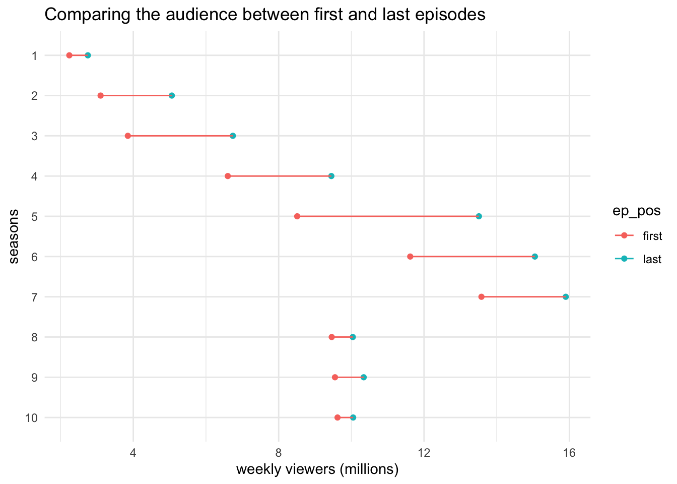
ep_df %>%
  group_by(series) %>%
  mutate( ep_pos = case_when(
    episode == max(episode) ~ "last",
    episode == min(episode) ~ "first",
    T ~ "other"
  )) %>%
  ungroup() %>%
  filter(ep_pos!="other") %>%
  select(ep_pos, series, viewers_7day) %>%
  ggplot(aes(x=viewers_7day, y=fct_rev(series), color=ep_pos, group=series))+
  geom_point() +
  geom_line() +
  theme_minimal()+
  labs(y="seasons", x="weekly viewers (millions)",
       title = "Comparing the audience between first and last episodes")
|
 1
 2
 3
 4
 5
 6
 7
 8
 9
10
11
12
13
14
15
16
17
18
19
20
21
22
23
24
25
26
27
28
29
30
|
ep_frst_lst <- ep_df %>%
  group_by(series) %>%
  mutate(ep_pos = case_when(
    episode == max(episode) ~ "last",
    episode == min(episode) ~ "first",
    T ~ "other"
  )) %>%
  ungroup() %>%
  filter(ep_pos != "other") %>%
  select(ep_pos, season=series, viewers_7day)

series_label <- ep_frst_lst %>%
  filter(ep_pos == "last")

p1 <- ep_frst_lst %>%  ggplot(
  aes(
    x = ep_pos,
    y = viewers_7day,
    color = season,
    group = season
  )
) +
  geom_point() +
  geom_line() +
  theme_minimal() +
  theme(legend.position = "none")+
  labs(x="episodes", y="weekly viewers (millions)",
       title = "Comparing the audience between first and last episodes")

p1 + geom_text(data=series_label,mapping= aes(x = ep_pos, y = viewers_7day, label = season),nudge_x = .1)
|

