“The only way to learn mathematics is to do mathematics.” - Paul Halmos. Taking time out of the day-to-day rush to finally learn how to use {tidymodels} for machine learning. These are the notebooks that I did to enter in this universe.
Better later than never. I take a time to finally learn how to use {tidymodels} for machine learning. Tidymodels is a set of packages that replaces the {caret} package as a ML framework to cover various aspects of the pipeline and try to standardizing the use of many different algorithms.
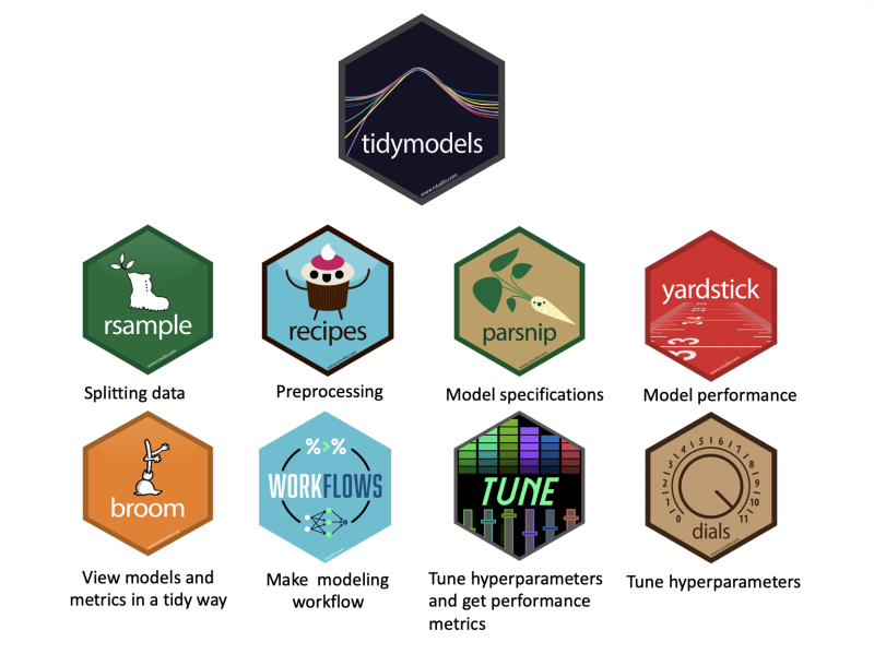
It’s powerful set of packages, but also with a very different APIs and design principles, so I have to stop and learn how to use doing some scripts to test the several packages of this universe. This one bellow is the “simplest case” and a put other cases in my GitHub.
tidymodels package set
The Simplest Pipeline
Intro
The simplest steps to make a straightforward ML pipeline using {tidyverse} packages follows these steps:
use {rsample} to split the dataset between training and testing subsets
use {recipes} to make some data preprocessing script
use {parsnip} to define a ranger random forest model
put the recipe and the model in a {workflow} object
library(tidymodels)library(mlbench)# mlbench is a library with several dataset to perform ML traininglibrary(skimr)# to look the dataset# loading "Boston Housing" datasetdata("BostonHousing")
Dataset: Boston Housing Dataset
Housing data contains 506 census tracts of Boston from the 1970 census. The dataframe BostonHousing contains the original data by Harrison and Rubinfeld (1979), the dataframe BostonHousing2 the corrected version with additional spatial information.
You can include this data by installing mlbench library or download the dataset. The data has following features, medv being the target variable:
crim - per capita crime rate by town
zn - proportion of residential land zoned for lots over 25,000 sq.ft
indus - proportion of non-retail business acres per town
chas - Charles River dummy variable (= 1 if tract bounds river; 0 otherwise)
nox - nitric oxides concentration (parts per 10 million)
rm - average number of rooms per dwelling
age - proportion of owner-occupied units built prior to 1940
dis - weighted distances to five Boston employment centers
rad - index of accessibility to radial highways
tax - full-value property-tax rate per USD 10,000
ptratio- pupil-teacher ratio by town
b 1000(B - 0.63)^2, where B is the proportion of blacks by town
lstat - percentage of lower status of the population
medv - median value of owner-occupied homes in USD 1000’s
1
2
BostonHousing%>%skim()
Table: Table 1: Data summary
Name
Piped data
Number of rows
506
Number of columns
14
_______________________
Column type frequency:
factor
1
numeric
13
________________________
Group variables
None
Variable type: factor
skim_variable
n_missing
complete_rate
ordered
n_unique
top_counts
chas
0
1
FALSE
2
0: 471, 1: 35
Variable type: numeric
skim_variable
n_missing
complete_rate
mean
sd
p0
p25
p50
p75
p100
hist
crim
0
1
3.61
8.60
0.01
0.08
0.26
3.68
88.98
▇▁▁▁▁
zn
0
1
11.36
23.32
0.00
0.00
0.00
12.50
100.00
▇▁▁▁▁
indus
0
1
11.14
6.86
0.46
5.19
9.69
18.10
27.74
▇▆▁▇▁
nox
0
1
0.55
0.12
0.38
0.45
0.54
0.62
0.87
▇▇▆▅▁
rm
0
1
6.28
0.70
3.56
5.89
6.21
6.62
8.78
▁▂▇▂▁
age
0
1
68.57
28.15
2.90
45.02
77.50
94.07
100.00
▂▂▂▃▇
dis
0
1
3.80
2.11
1.13
2.10
3.21
5.19
12.13
▇▅▂▁▁
rad
0
1
9.55
8.71
1.00
4.00
5.00
24.00
24.00
▇▂▁▁▃
tax
0
1
408.24
168.54
187.00
279.00
330.00
666.00
711.00
▇▇▃▁▇
ptratio
0
1
18.46
2.16
12.60
17.40
19.05
20.20
22.00
▁▃▅▅▇
b
0
1
356.67
91.29
0.32
375.38
391.44
396.22
396.90
▁▁▁▁▇
lstat
0
1
12.65
7.14
1.73
6.95
11.36
16.96
37.97
▇▇▅▂▁
medv
0
1
22.53
9.20
5.00
17.02
21.20
25.00
50.00
▂▇▅▁▁
We’ll try to predict medv (median value of owner-occupied homes).
recp<-BostonHousing%>%recipe(medv~.)%>%# formula goes herestep_nzv(all_predictors(),-all_nominal())%>%# remove near zero varstep_center(all_predictors(),-all_nominal())%>%# center step_scale(all_predictors(),-all_nominal())%>%# scalestep_BoxCox(all_predictors(),-all_nominal())# box cox normalizationrecp
1
2
3
4
5
6
7
8
9
10
11
12
13
14
## Data Recipe
##
## Inputs:
##
##       role #variables
##    outcome          1
##  predictor         13
##
## Operations:
##
## Sparse, unbalanced variable filter on all_predictors(), -all_nominal()
## Centering for all_predictors(), -all_nominal()
## Scaling for all_predictors(), -all_nominal()
## Box-Cox transformation on all_predictors(), -all_nominal()
# the do all by itself# calculates the data preprocessing (recipe)# apply to the training set# fit the model using itmodel_fit<-fit(wf,training(boston_split))model_fit
# the prediction applied on the fitted automatically# apply the trained transformation on the new dataset# and predict the output using the trained modely_hat<-predict(model_fit,testing(boston_split))head(y_hat)
library(tidymodels)library(mlbench)# mlbench is a library with several dataset to perform ML traininglibrary(skimr)# to look the dataset# loading "Boston Housing" datasetdata("BostonHousing")# data overviewBostonHousing%>%skim()# split boston_split<-initial_split(BostonHousing)# recipe: preprocessing scriptrecp<-BostonHousing%>%recipe(medv~.)%>%# formula goes herestep_nzv(all_predictors(),-all_nominal())%>%# remove near zero varstep_center(all_predictors(),-all_nominal())%>%# center step_scale(all_predictors(),-all_nominal())%>%# scalestep_BoxCox(all_predictors(),-all_nominal())# box cox normalization# Model Specificationmodel_eng<-rand_forest(mode="regression")%>%set_engine("ranger")# Workflowwf<-workflow()%>%add_recipe(recp)%>%# preprocessing specification (with formula)add_model(model_eng)# model specification# Training the model with workflow# the do all by itself calculates the data preprocessing (recipe)# apply to the training set fit the model using itmodel_fit<-fit(wf,training(boston_split))# Predicty_hat<-predict(model_fit,testing(boston_split))head(y_hat)# Evaluatey_hat%>%bind_cols(testing(boston_split))%>%# binds the "true value"metrics(truth=medv,estimate=.pred)# get the estimation metrics (automatically)